Loss-Free MoE Routing

Overview: In this post I explore two criteria for MoE routers—load balancing and geometric conditioning—and propose two new methods. The first uses Manifold Muon to keep the router perfectly conditioned throughout training. The second is a single update rule that achieves load balancing and orthogonality with no auxiliary balancer and is detached from the training loss entirely. Both train stably, stay well balanced and perfectly conditioned, and suggest a broader family of loss-free router optimizers.

What’s in a router?

(1) Load Balancing

A standard transformer has one MLP per layer. A mixture-of-experts (MoE) model has many, each called an expert, but routes each token to only a few of them. The routing decision is controlled by an $E\times D$ weight matrix (the router), where each row is a single expert’s selection vector.

Each expert owns a single row in the router matrix, which is just a point in activation space. Tokens arrive with their own activations, and routing scores are decided based on the similarity between experts’ vectors and token activations. In a simplified model where all these vectors are unit-normalized, each token routes to its nearest expert.

A router balancer modifies the effective catchment radius around each expert so that each receives a near-equal number of tokens.

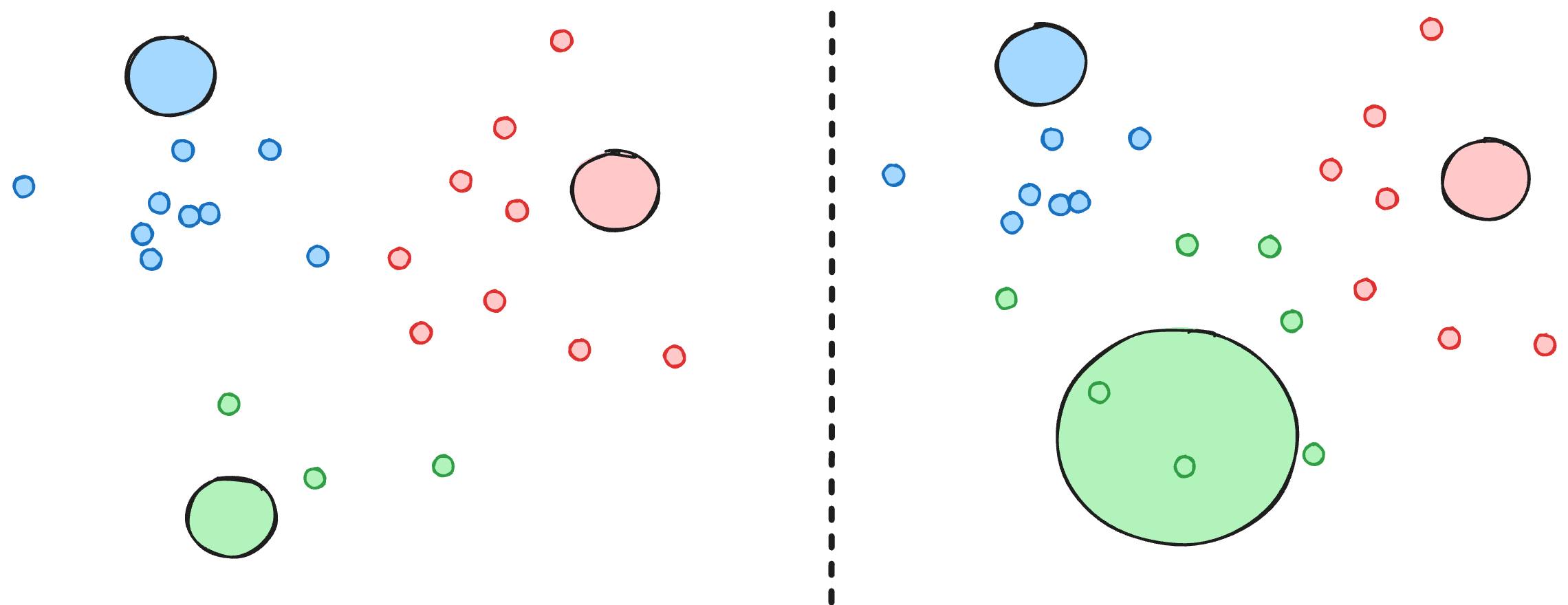
Figure 1: A simplified setup with 3 experts. The large circles represent three routing vectors and the small dots are colored by assignment. (Left) unbalanced routing, where the green expert receives only a few tokens. (Right) we expand the effective radius of the green expert, and now each expert receives a near-equal share of tokens.

Without balancing you will end up in a vicious feedback loop of dead experts.¹ If an expert receives fewer tokens, it will become undertrained, which will encourage the router to continue diverting tokens away from this expert.

To promote balance, GShard² (2020) added an auxiliary loss function that measures how imbalanced the experts are. This is simple to implement, since the autograd framework handles the complexities of how each expert should become balanced. The problem is that your model now has two objectives that can conflict with each other:

Existing methods commonly employ an auxiliary loss to encourage load balance, but a large auxiliary loss will introduce non-negligible interference gradients into training and thus impair the model performance. Although the auxiliary loss can alleviate load imbalance during training, it also introduces undesired gradients that conflict with the language modeling objective.

The above quote is from DeepSeek³, who chose to drop the auxiliary loss entirely. Instead of optimizing a second objective, they adjust the radius around each expert using a learnable scalar bias. Subsequent work like SMEBU⁴ and Quantile Balancing⁵⁶ modify the dynamics by which these biases are learned.

Each approach confers different dynamics over the course of training, though all are effective⁷:

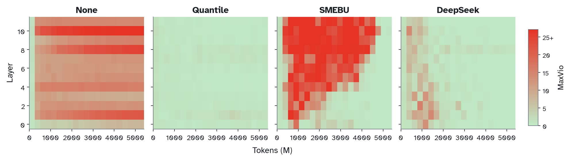
Figure 2: Load balancing throughout the duration of training as measured by MaxVio: how much the most overloaded expert’s token share is above its balanced allocation. All load-balancing techniques result in zero dead experts by the end of training.

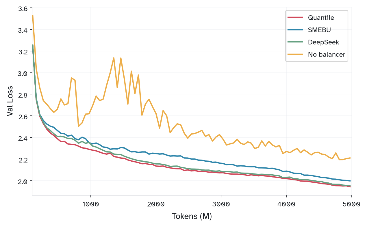
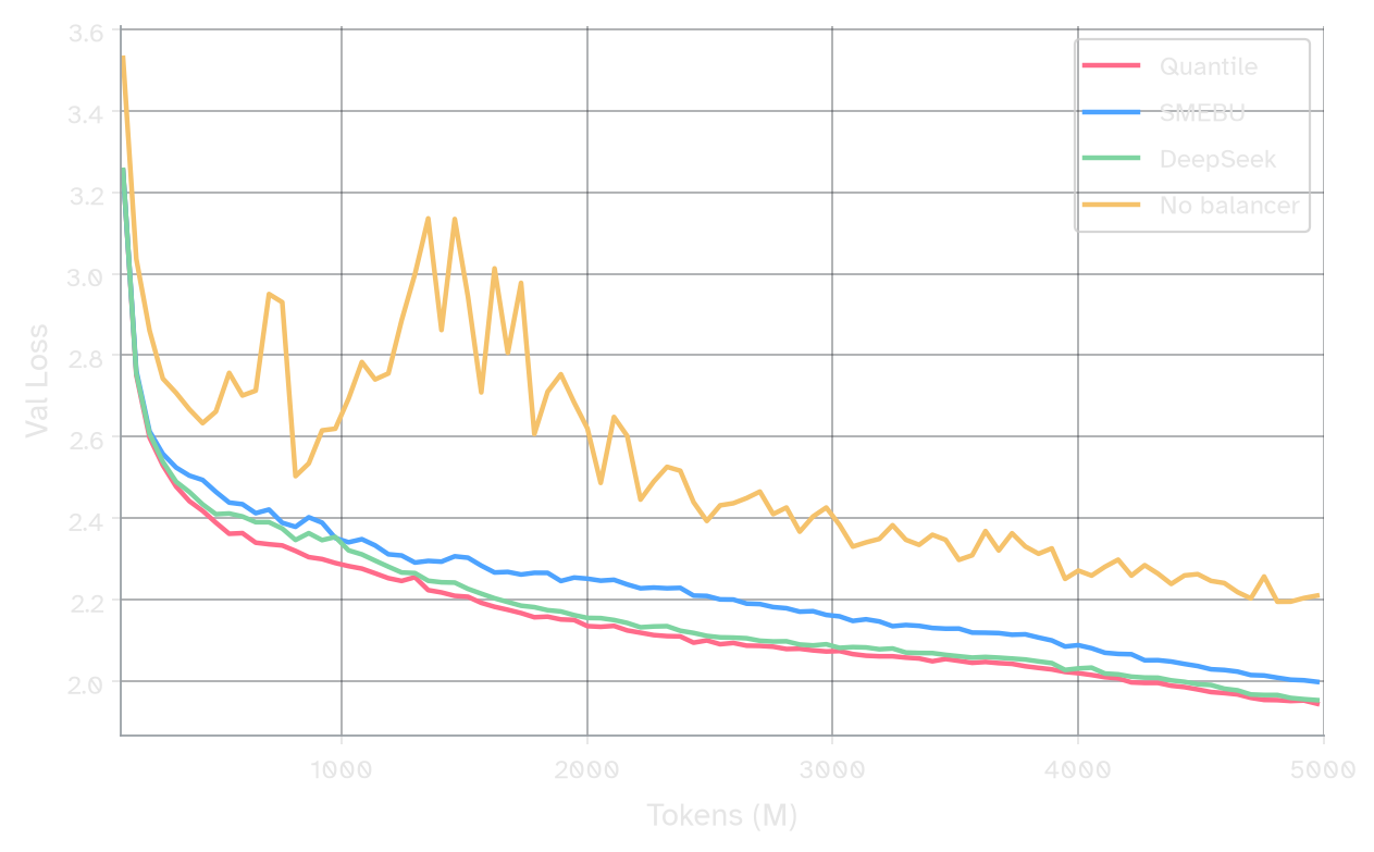
Figure 3: Validation loss trajectories for each load balancing method.

(2) Stability and Conditioning

For the results in Part 1, I used Adam on the routers. At first glance, Muon seems like a poor fit for the MoE Router.

Unlike a regular linear layer, the MoE router’s rows are structurally independent: each row’s gradient comes only from the tokens routed to that expert. But the gradient produced by backprop is not directly applied to the router; it is transformed first by the optimizer. While Adam respects this rowwise independence, Muon doesn’t. This is apparent when considering the Shampoo update rule:

def shampoo_update(G, L, R, W, lr):
	L = L + G @ G.mT
	R = R + G.mT @ G
	return W - lr * (L^{-1/4} @ G @ R^{-1/4})

Algorithm 1: Simplified shampoo update. Barring details on accumulation and approximation, the above is identical to Muon.⁸⁹ The L factor blends gradient signals across rows. Expert $j$‘s update is contaminated by expert $i$‘s gradient, even though the two never share tokens.

I found this rowwise violation deeply distressing! However, while testing, I found Muon is not much worse than Adam on the router:

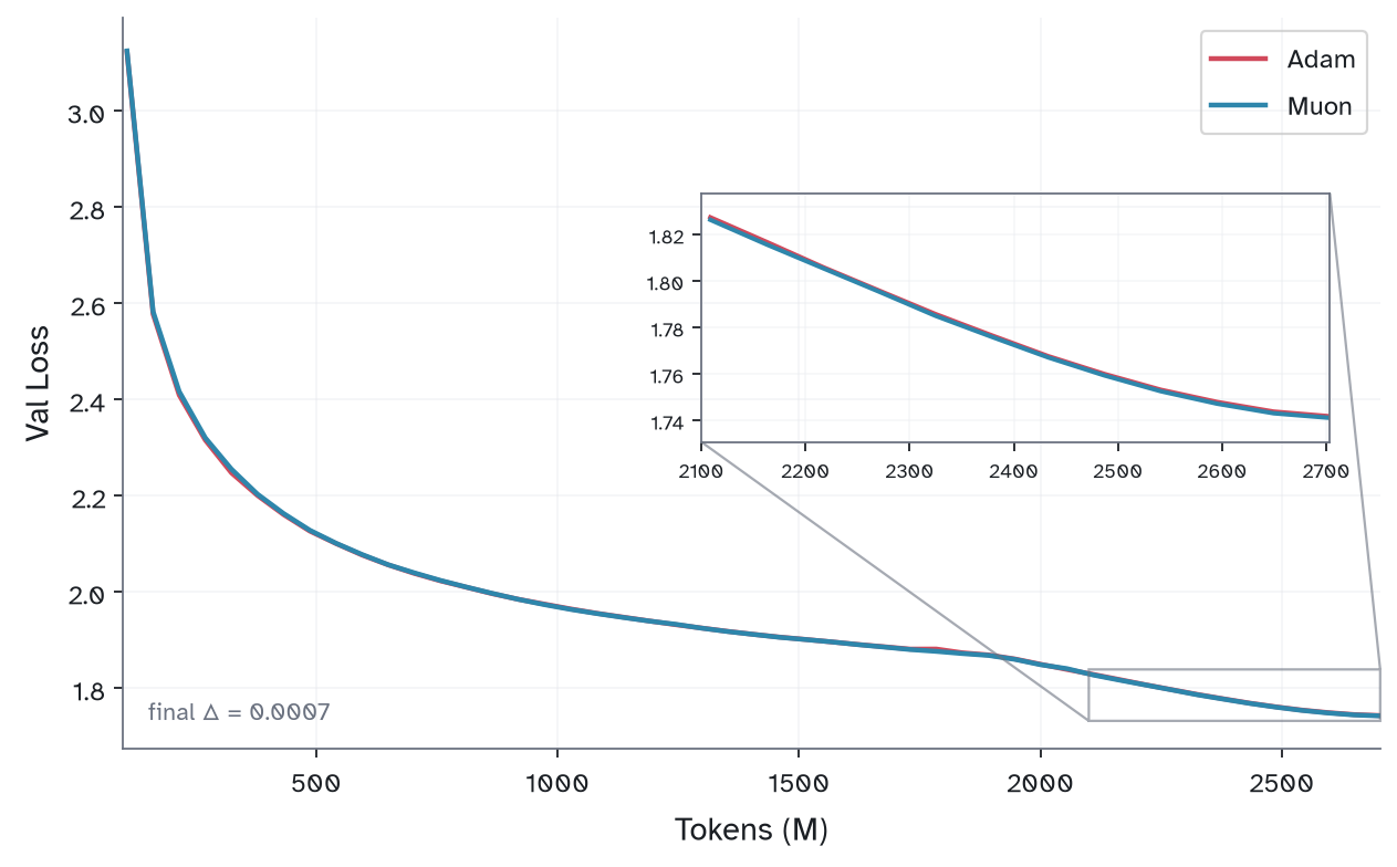
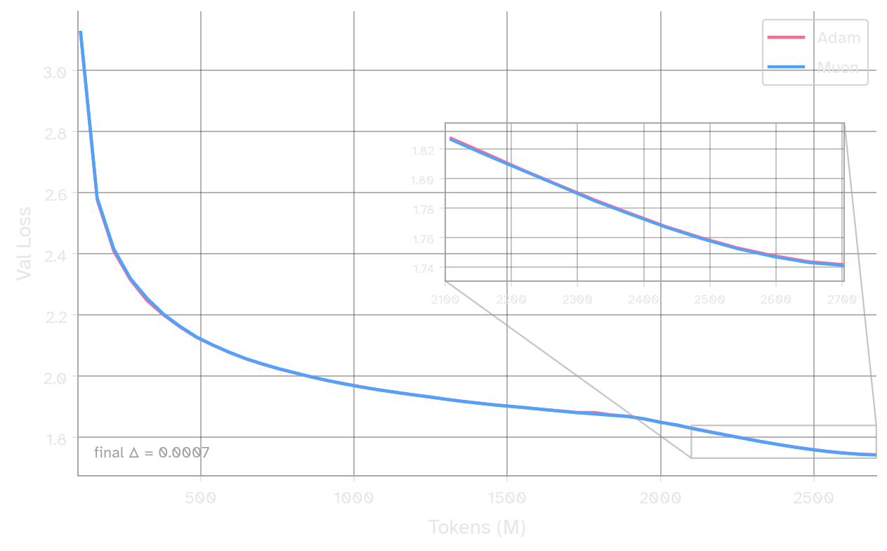
Figure 4: Validation loss of Adam vs Muon used on the MoE router. Muon is nearly identical throughout training.

If validation loss is no better, why bother with Muon? The Moonshot AI team used Muon on the MoE router in the training of Kimi K2¹⁰¹¹ (and perhaps later models). They motivate this decision by showing that Muon produces a router with consistently higher SVD Entropy than Adam.

SVD Entropy is a metric that quantifies roughly what percent of expert routing vectors point in genuinely distinct directions. A router with high SVD Entropy is said to be well-conditioned. A poorly-conditioned router will have many rows that are in the span of other rows, which means that these rows have no discriminative power, since they do not point to unique directions in feature space. In the extreme case, two experts with identical routing vectors receive statistically indistinguishable sets of tokens, train on the same inputs, and likely converge toward the same function.

For small-scale experiments, especially for extremely sparse models, conditioning may be a more useful measure than val loss. In the above experiments, the model has roughly 1.5B total parameters trained on 2.7B tokens — about 1.8 tokens per parameter. At this budget, expert specialization is probably not truly meaningful since the underlying data may not be diverse enough to reflect genuinely useful distinctions.

Condition number is especially useful for measuring the quality of the router since this weight is discontinuous under top-$k$: small drifts in the weight matrix cause discrete jumps in token assignment.

I found Muon greatly improves the conditioning of the router weights:

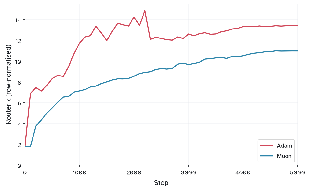
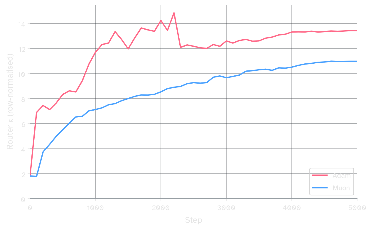
Figure 5: Router condition number $\kappa ={\sigma }_{\max }/{\sigma }_{\min }$ is an extremal measure of conditioning, where a perfectly conditioned matrix has condition number $1$. Unlike SVD Entropy, which is a measure of average conditioning, a low $\kappa$ bounds the worst-case amount of redundancy in the router. Muon produces a better-conditioned router than Adam throughout the duration of training.

So Muon is roughly net even on loss but improves conditioning. The simple intuition is that Muon’s individual updates have perfect conditioning (orthogonalization), and therefore the accumulation of all of these updates also has very good conditioning, though further exposition of this phenomenon is given in additional work.¹²

Two new methods

(3) Manifold Optimization

In the previous section, we found that Muon achieves better geometric conditioning of the routers than Adam. Here, I want to explore what happens when we target perfect conditioning.

For the router matrix, the conditioning is perfect if and only if all rows are orthogonal with equal norm. This property, rowwise orthogonality, has a useful interpretation for the router specifically. When two routing vectors have high cosine similarity, there exists a subspace where tokens are indistinguishable to those experts, and any token in that subspace gets assigned between them essentially at random. Rowwise orthogonality ensures no two routing vectors are redundant, and that small perturbations to the router weight do not severely change routing dynamics. Better orthogonality, which corresponds to better conditioning, may end up producing a much healthier model on a variety of downstream metrics when fully trained.

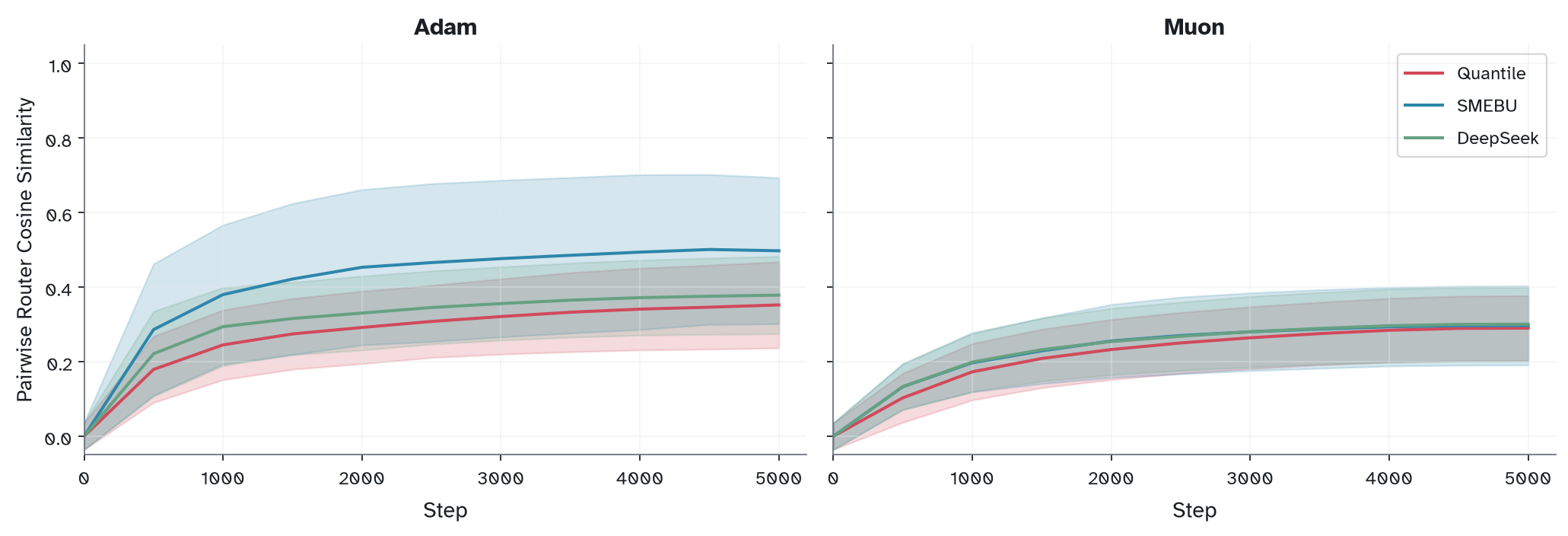
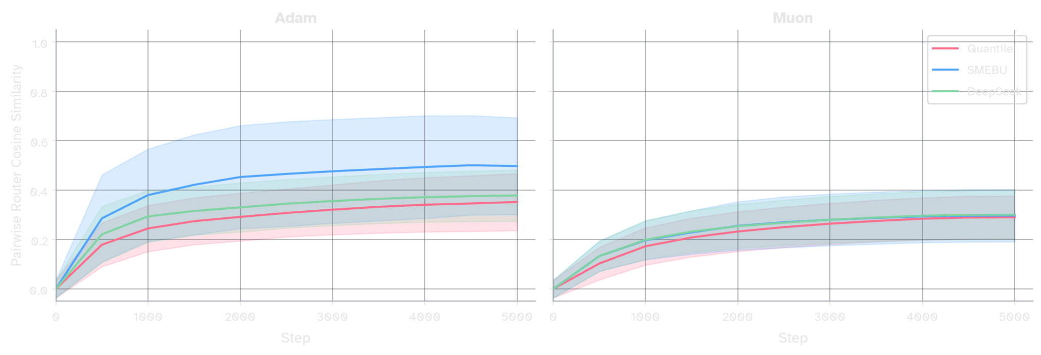
Figure 6: Mean pairwise cosine similarity between router rows over training. Adam (left) vs Muon (right) across the three balancing methods mentioned previously (Quantile, SMEBU, Deepseek). Muon produces more pairwise-orthogonal router than Adam.

Several recent works¹³¹⁴¹⁵ have defined an aux loss for the MoE router that explicitly encourages rowwise orthogonalization:

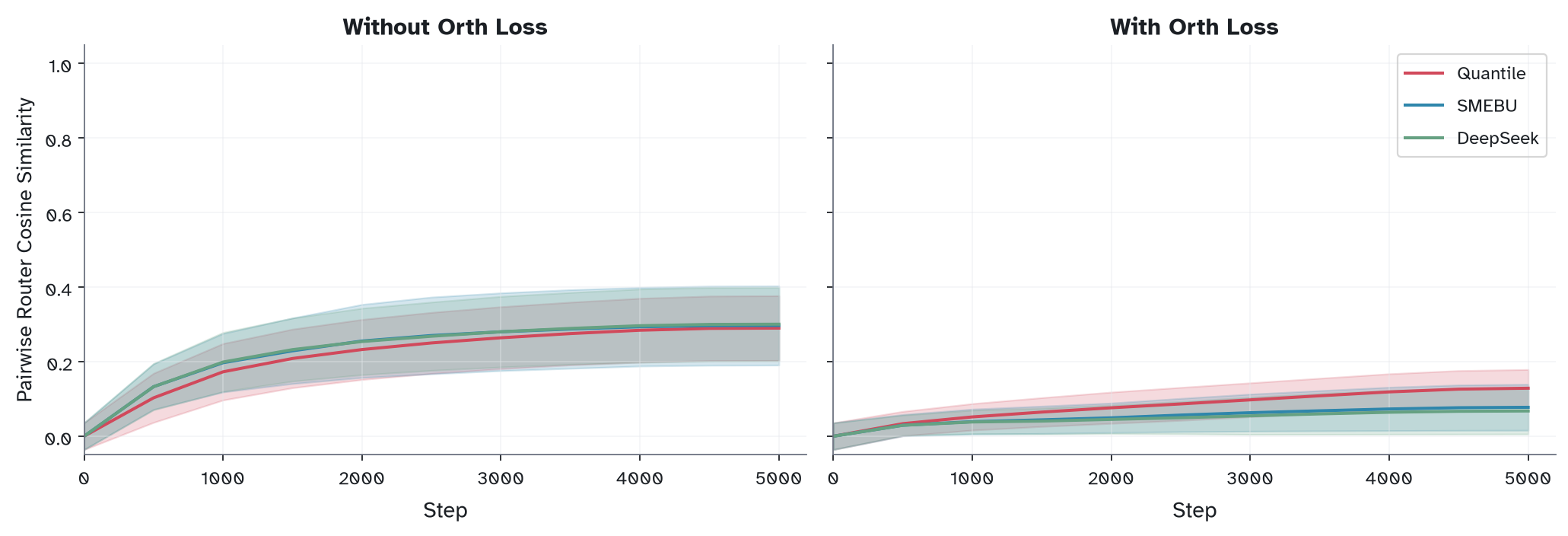
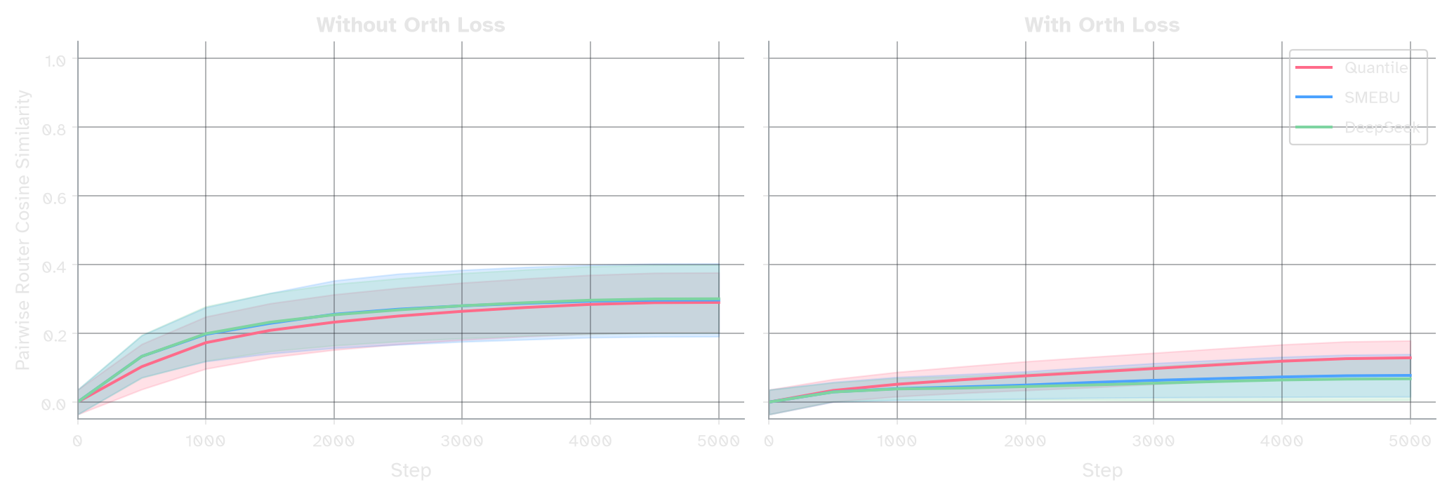
Figure 7: Mean pairwise cosine similarity under Muon without (left) and with (right) the orthogonalization auxiliary loss (in this case, as proposed by Baidu’s ERNIE team). The orth loss drives similarities lower, though they remain nonzero and growing.

Rather than encouraging orthogonality, we can enforce it directly. In 2025, Jeremy Bernstein¹⁶ proposed Manifold Muon, in which weights are constrained to the Stiefel Manifold. For router weights, where the number of experts is less than the hidden dimension, this gives us exact rowwise orthogonality.

def sym(X: Tensor) -> Tensor:
    return 0.5 * (X + X.mT)
    
def manifold_muon_update(
    W: Tensor, G: Tensor, lr: float,
    dual_lr: float = 0.01, dual_steps: int = 100,
) -> Tensor:
    G = G / (G.norm() + 1e-8)
    # init Lambda so first iterate ≈ tangent_project(G, W)
    Lambda = -0.5 * sym(G @ W.mT)
    # dual ascent
    for i in range(dual_steps):
        Z = msign(G + 2 * sym(Lambda) @ W)
        Lambda -= dual_lr * (1 - i / dual_steps) * sym(Z @ W.mT)
    # update, retract
    vel = msign(G + 2 * sym(Lambda) @ W)
    return msign(W - lr * vel)

Algorithm 2: Manifold Muon. msign is the matrix sign function (Newton-Schulz / Polar Express). This code assumes W is wide (W.shape[0] <= W.shape[1]). For full implementation details see the Appendix.

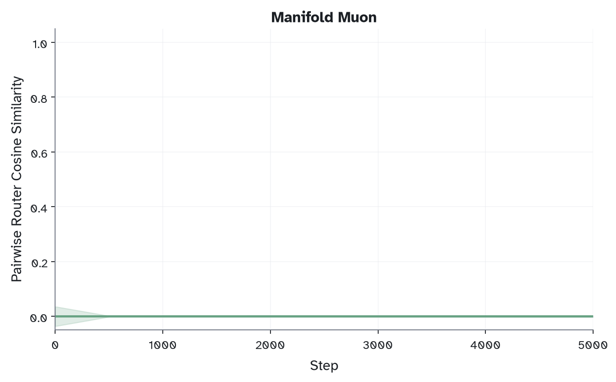
Simply swapping out Muon for Manifold Muon on the router gives us a router with perfectly orthogonal rows throughout training: 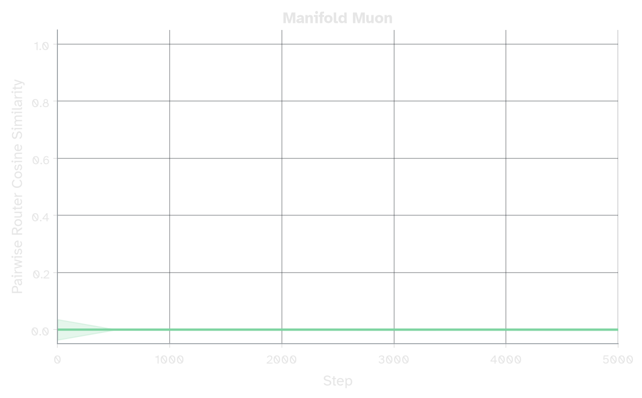Figure 8: Mean pairwise cosine similarity under Manifold Muon. Rows remain exactly orthogonal throughout training.

Moreover, I found the validation loss to be comparable, though slightly worse, than Adam and Muon.

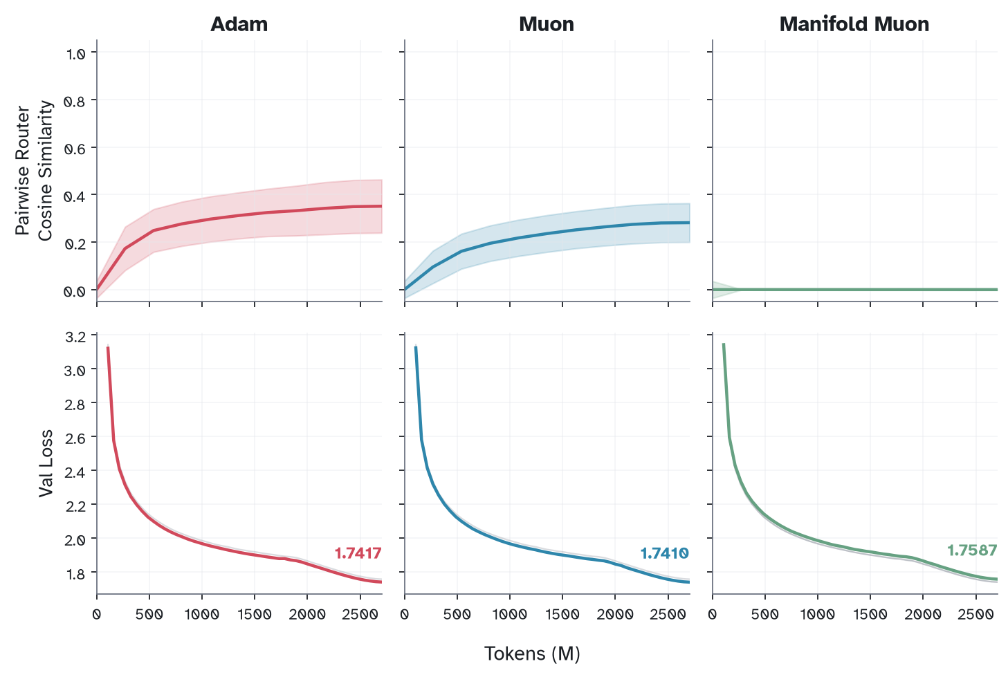
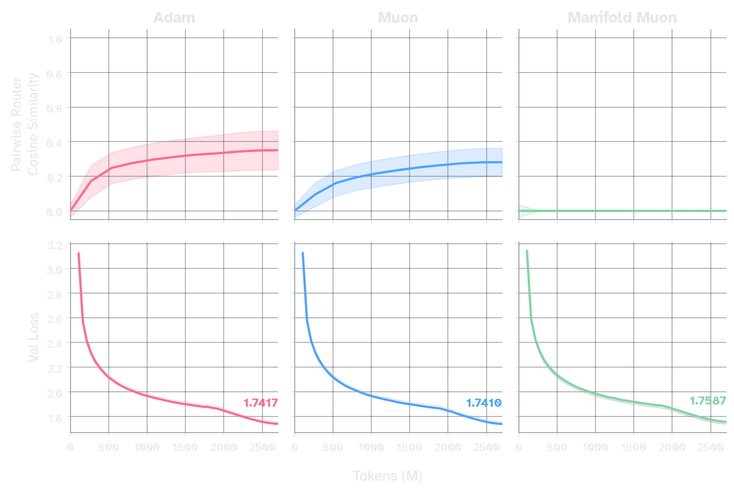
Figure 9: Pairwise cosine similarity (top) and validation loss (bottom) over training for Adam, Muon, and Manifold Muon. Perfect orthogonality costs a bit of val loss.

(4) Loss-Free Routing

One of the surprising results from the previous two sections is that Muon’s gradient row-mixing doesn’t hurt val loss too much. This suggests that respecting the cross-entropy gradient isn’t crucial toward training our router.

The implicit assumption so far has been that each routing row learns to select tokens whose features its expert is good at processing. I’d like to reverse this assumption by training a router that knows nothing about its downstream experts, and instead allowing the experts to learn to process whatever tokens they receive.

Orthogonality can be understood as a data-agnostic approximation to capacity: a measure of how much of the incoming token distribution we cover. Recalling the nearest-neighbors formulation from Part 1, we’d like for the majority of incoming tokens to be contained within the span of the routing vectors. An orthogonal router is also a perfectly conditioned one: following the logic from Part 2, each routing vector points in a unique direction, giving the router the most discriminative power possible.

If token activations were uniformly distributed on the sphere (in ${\mathbb{R}}^d$), orthogonal routing vectors would maximize capacity exactly. They aren’t uniform (if they were, load balancing would also be trivial), so maximizing the routing simplex isn’t the same as maximizing capacity. Orthogonality is a naive but principled starting point, as the max-volume geometry when you ignore incoming token distribution. Load balancing and orthogonality can be thought of as complementary aspects toward capacity maximization.

Recall that the primary motivation of aux-loss-free load balancing was the conflict between two objectives’ distinct gradients. DeepSeek’s loss-free balancing dropped the auxiliary loss and kept the LM gradient. What if we try the opposite approach? We can design an optimizer where structural orthogonality and load-balancing are the only tools we have to maximize capacity. First, we calculate the exact update needed to balance the experts based on the incoming token stream. Then, we feed this update into Manifold Muon before applying it to the router.

def loss_free_router_step(W, x, logits, lr):
    # 1. balancing gradient (see Appendix for derivation)
    rho = torch.sigmoid(logits)
    F = rho.mean(dim=0)
    s = rho * (1 - rho)
    scale = (2.0 / x.shape[0]) * (F - F.mean())
    G = scale.unsqueeze(1) * (s.T @ x)
    # 2. manifold muon update
    return manifold_muon_update(W, G, lr)

The routers receive no other updates, neither from the typical backprop update nor from any additional load balancer. Full details + code are in the Appendix, but here are the results. First, orthogonality, guaranteed by construction, gives us perfect conditioning.

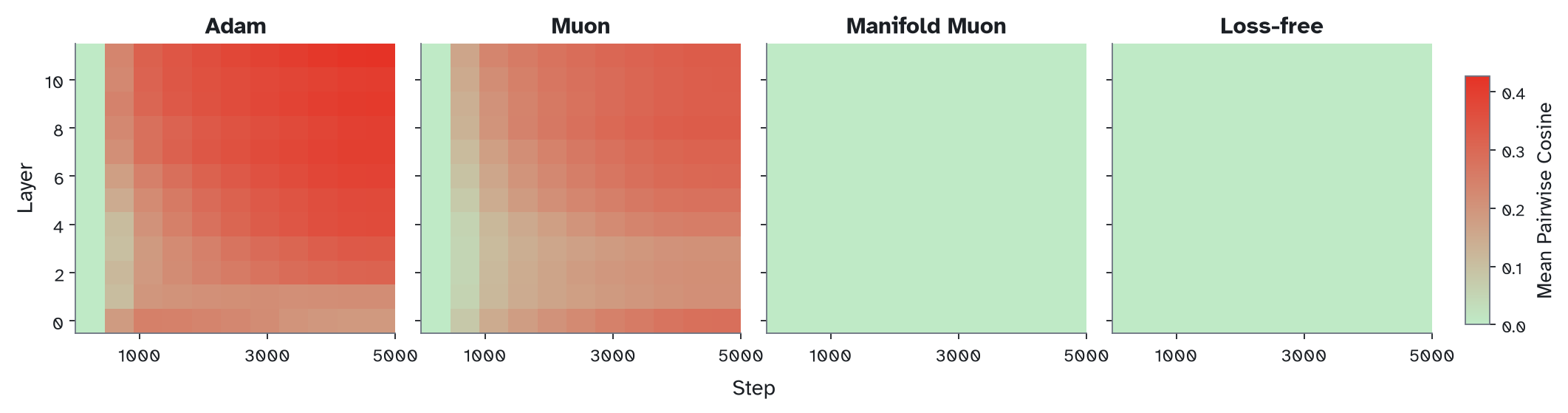
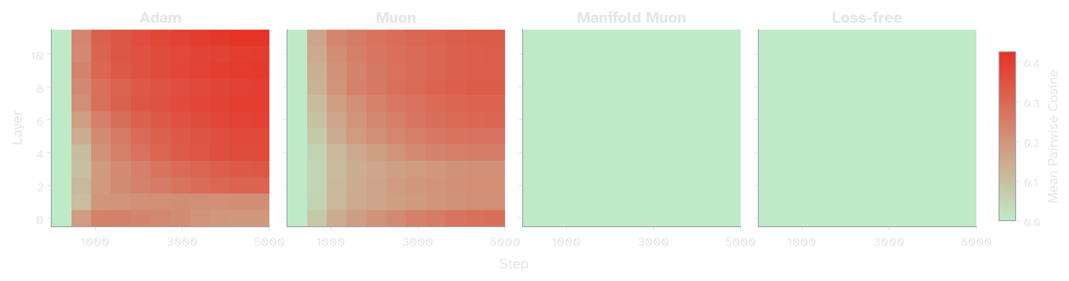
Figure 10: Mean pairwise cosine similarity by layer over training for all four router optimizers. Adam and Muon accumulate similarity in later layers; Manifold Muon and the loss-free router maintain near-zero similarity throughout.

The loss-free update rule also guarantees balance, and it is achieved with the same efficacy as methods with auxiliary balancers.

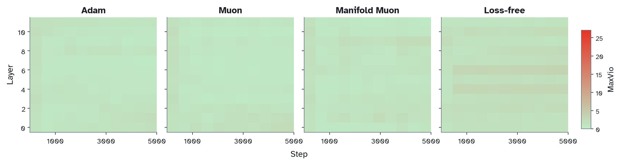
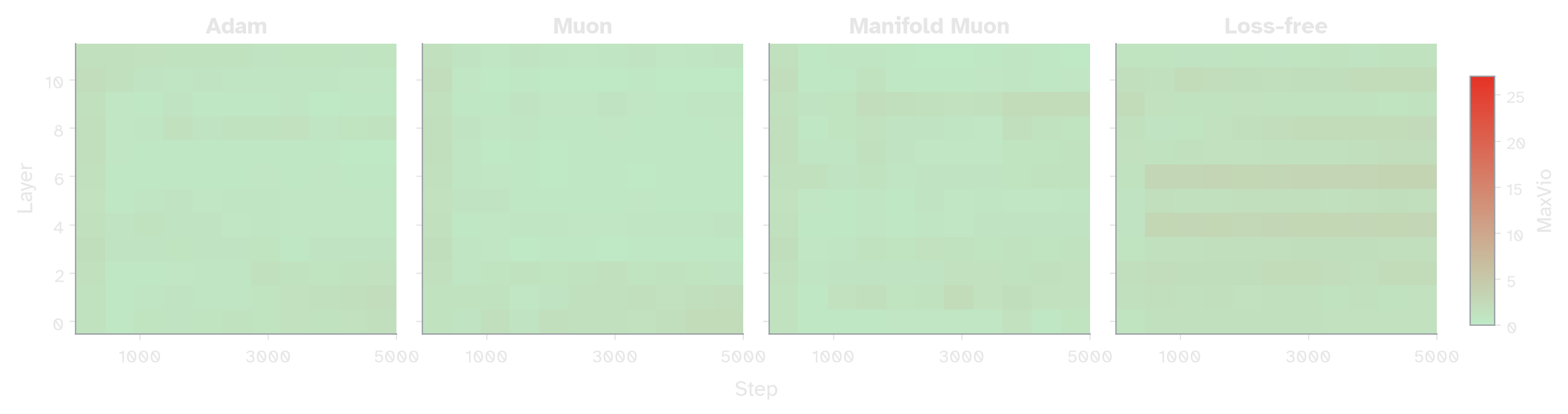
Figure 11: MaxVio by layer over training for the Loss-free router (rightmost) versus previous methods (Adam, Muon, Manifold Muon with Quantile Load Balancer). Even with no external balancer, MaxVio is low throughout training.

Finally, we find that validation loss for loss-free routing lags behind, though it is not disastrous.

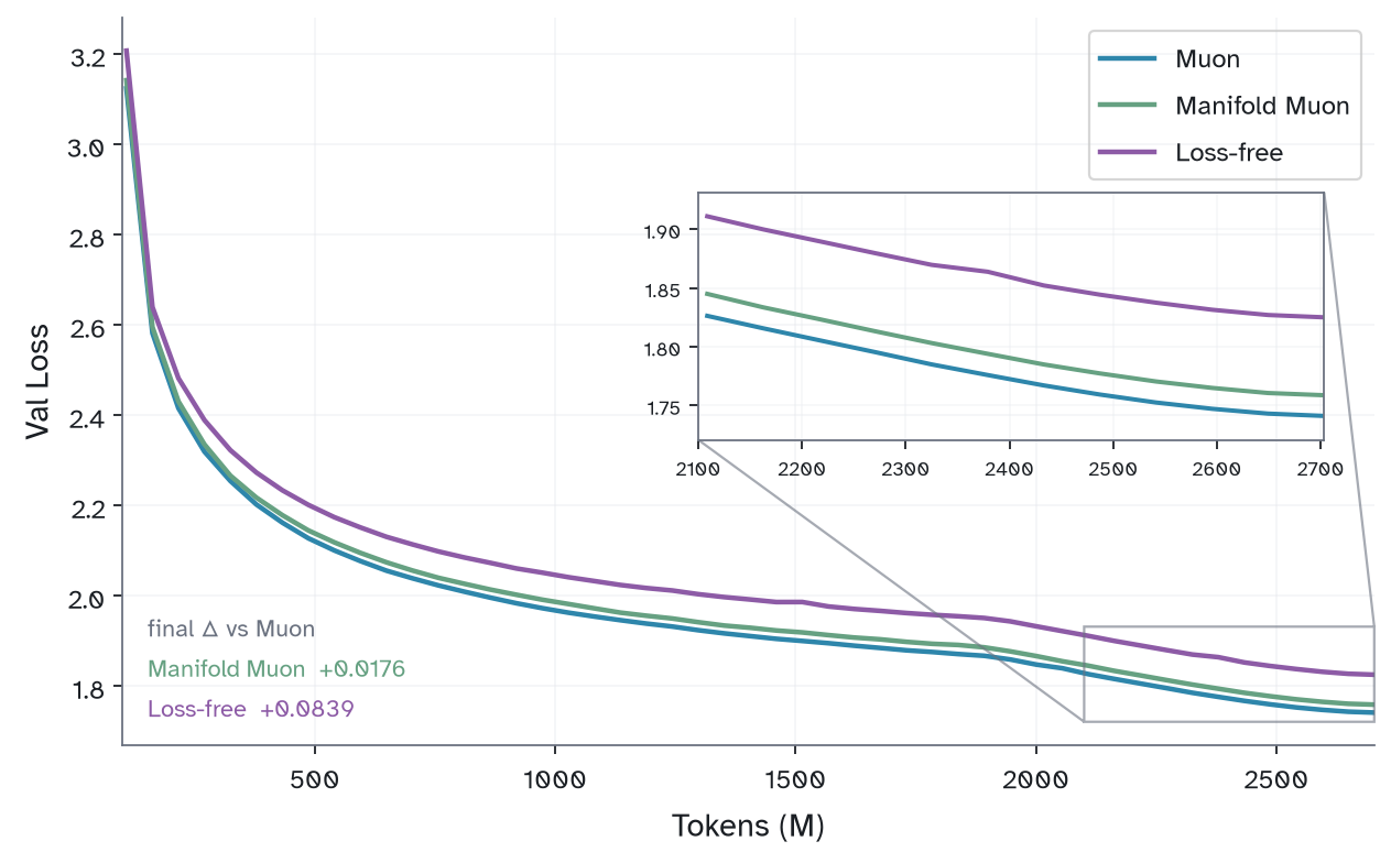
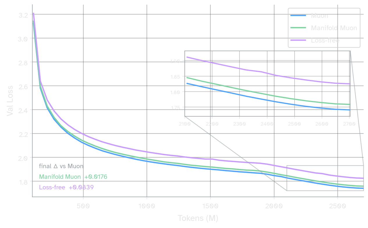
Figure 12: Validation loss under loss-free routing compared to previous methods. Training is stable and monotonic, though val loss lags behind.

The router achieves perfect orthogonality and balance with no gradient from the LM head. The validation loss lags behind the previous implementations, but training still appears to be monotonic and stable.

Why bother?

Since this section’s approach lags behind in validation loss, it’s clear that the training loss is useful for something. On the other hand, it doesn’t appear to be strictly necessary for training mixture-of-experts models. Initial research on MoEs encouraged balance with auxiliary loss functions; later work swapped these for learnable biases, then for bespoke bias-update rules, each a progressively lighter intervention.

I believe the most principled version of MoE training is not composed of several distinct update functions; rather, a single criterion combined with a single optimizer, which matches how every single other parameter in the transformer is trained. The proposed method in this section is one instance of this: gradient descent on the load-balancing criterion combined with a geometrically-structured optimizer (Manifold Muon).

Typically, gradient descent is very powerful. To some extent, over-engineering the router is in violation of our natural trust in its power. As Karpathy wrote in 2017, gradient descent can write code better than you.¹⁷ Routing is discontinuous under top-$k$, which makes the router the one component of the transformer for which cross-entropy is an awkward criterion. I don’t think the problem is descent; rather, what we choose to descend.

My suspicion is that the final criterion will end up remarkably simple, though it may not look exactly like load balancing. As indicated earlier, this method seems to be a data-agnostic approximation to capacity. It may be possible to simply write down a single criterion that maximizes capacity, and to optimize for this directly.

---

Appendix

Derivation and Code

def sym(X: Tensor) -> Tensor:
    return 0.5 * (X + X.mT)
 
def manifold_muon_update(
    W: Tensor, G: Tensor, lr: float,
    vel_ema: Tensor | None = None, beta: float = 0.9,
    mu: float = 1.0, admm_steps: int = 20, preserve_mag: bool = True,
) -> Tensor:
    # step-size gate: preserves balance signal
    mag = torch.tanh(G.norm()) if preserve_mag else 1.0
    G = G / (G.norm() + 1e-8)
    # init Lambda so first iterate ≈ tangent_project(G, W)
    Lambda = -0.5 * sym(G @ W.mT)
    Z = G + 2 * Lambda @ W
    Omega = torch.zeros_like(Z)
    eye = torch.eye(W.shape[0], device=W.device, dtype=W.dtype)
    # ADMM
    for _ in range(admm_steps):
        Lambda = 0.5 * sym((Z + Omega / mu - G) @ W.mT)
        B = G + 2 * Lambda @ W - Omega / mu
        P_pos = 0.5 * (eye + msign(B @ B.mT - eye / mu**2))
        Z = P_pos @ (B - msign(B) / mu)
        Omega += mu * (Z - G - 2 * Lambda @ W)
    # tangent velocity
    vel = msign(G + 2 * sym(Lambda) @ W)
    vel = tangent_project(-lr * mag * vel, W)
    # momentum
    if vel_ema is not None:
        vel_ema.lerp_(vel, 1 - beta)
        vel = tangent_project(vel_ema, W)
    # retract to Stiefel manifold
    return streaming_msign(W + vel)

Algorithm 3: The full Manifold Muon update used in my experiments, with an ADMM inner solver, momentum on the tangent velocity, and an optional magnitude gate. Each trick is detailed below.

Useful details:

• The inner loop uses ADMM to solve the constrained optimization over the Stiefel manifold.¹⁸ This reformulation by Buchanan drops the required inner-loop iterations by an order of magnitude compared to Bernstein’s original dual-ascent solver.
• I found convergence is better (especially for the Loss Free method) when the input gradient is considered (which would typically be discarded under Manifold Muon). I gate the step size as $\tanh (|G|)$ and use it to scale the update. This simple heuristic is not needed but helpful for convergence.
• msign uses Polar Express in fp16 (more numerically stable than bf16)
• streaming_msign uses Jianlin Su’s Streaming SVD¹⁹ algorithm. The reason for this is to encourage the final msign to have the same order of singular vectors from step-to-step. Newton-Schulz (and similar algorithms) may noisily shuffle rows in early training, which is dangerous for routing weights.
• I’ve included logic that allows for momentumization to the retraction vector to the Stiefel Manifold (vel -> vel_ema). As far as I know, this addition is novel to the Manifold Muon literature. In my testing, this far outperforms momentumization of the incoming gradient signal.
• The router is initialized on the Stiefel manifold via torch.nn.init.orthogonal_.
• Routers of the same shape are batched into a single ADMM/msign call.

For the Loss Free optimizer, we use a classic balancing loss criterion, but compute its gradient explicitly rather than through autograd.

Let $W\in {\mathbb{R}}^{E\times D}$ be the router weight, with rows $W_j$ corresponding to each expert’s routing vector. Given token activations $x_1,\dots ,x_T\in {\mathbb{R}}^D$, the routing score for token $i$ to expert $j$ is ${\rho }_{i,j}:=\sigma (x_i\cdot W_j)$, where $\sigma$ is the sigmoid.²⁰ The mean routing score per expert is $F_j:=\frac{1}{T}{\sum }_{i=1}^T{\rho }_{i,j}$, and $F=[F_1,\dots ,F_E]\in {\mathbb{R}}^E$ is the vector of all expert loads.

Since $F$ is just a vector, we can understand its properties by comparing it against a target vector. If we want to ask how balanced $F$ is, we should compare it to $U=[\bar{F},\bar{F},\dots \bar{F}]$ where $\bar{F}$ is the mean value of $F$. This motivates a simple loss function like $\mathcal{L}(F)=||F-U|{|}^2$.

We want $\frac{\partial \mathcal{L}}{\partial W_j}$. By the chain rule:

$$\frac{\partial \mathcal{L}}{\partial W_j}=\frac{\partial \mathcal{L}}{\partial F_j}\cdot \frac{\partial F_j}{\partial W_j}$$

For the first term, since $\mathcal{L}=|F-U{|}^2={\sum }_k(F_k-\bar{F}{)}^2$ and ${\sum }_k(F_k-\bar{F})=0$:

$$\frac{\partial \mathcal{L}}{\partial F_j}=2(F_j-\bar{F})$$

For the second term, since $F_j=\frac{1}{T}{\sum }_i\sigma (x_i\cdot W_j)$ and ${\sigma }^{\prime }=\sigma (1-\sigma )$:

$$\frac{\partial F_j}{\partial W_j}=\frac{1}{T}\sum _{i=1}^T{\rho }_{i,j}(1-{\rho }_{i,j})x_i$$

Combining:

$$\boxed{\frac{\partial \mathcal{L}}{\partial W_j}=2(F_j-\bar{F})\cdot \frac{1}{T}\sum _{i=1}^T{\rho }_{i,j}(1-{\rho }_{i,j})x_i\in {\mathbb{R}}^D}$$

The full gradient ${\nabla }_W\mathcal{L}\in {\mathbb{R}}^{E\times D}$ stacks these rows. In matrix form, let $S=\rho \odot (1-\rho )\in {\mathbb{R}}^{T\times E}$:

$${\nabla }_W\mathcal{L}=\frac{2}{T}\text{diag}(F-\bar{F})S^{\top }X$$

This gives the Loss Free update from earlier.

def loss_free_router_step(W, x, logits, lr):
    # 1. balancing gradient 
    rho = torch.sigmoid(logits)
    F = rho.mean(dim=0)
    s = rho * (1 - rho)
    scale = (2.0 / x.shape[0]) * (F - F.mean())
    G = scale.unsqueeze(1) * (s.T @ x)
    # 2. manifold muon update
    return manifold_muon_update(W, G, lr)

This update rule converges rapidly as load balancing is achieved. As such, only updating every $n$ steps is probably sufficient.

Extensions

The loss-free method here used just one update rule (balance) and one geometric constraint (Stiefel).²¹ Both can be swapped. The balancing gradient can be replaced or augmented with any objective we can differentiate through the router, such as capacity-maximization (see the note on capacity in Section 4), sequence-level load balancing, or a domain specialization loss.

On the geometry side, strict orthogonality may be too aggressive when the number of experts is large. A natural relaxation is to target low coherence, a measure of how orthogonal a set of unit vectors is.²² Progressive relaxations of the Stiefel constraint are explored in Gram-Space Manifold Muon.²³

This whole philosophy of optimizing only a single criterion is inspired by my research into PSGD. The manifold retraction constraint resembles a PSGD preconditioner criterion. I believe both the design of the optimal criterion (e.g. capacity) and of the optimizer (e.g. geometric constraints) might be best understood through the framework of PSGD.

As a practical matter, the manifold update doesn’t need to run every step; skipping every $n$ steps is sufficient (see results above). Further optimizations include batching manifold Muon across layers, computing the balancing gradient during routing (no extra forward pass), and writing the result to .grad in order to reuse the normal gradient accumulation and all-reduce pipeline.

The experiments here are at small scale (12-layer, 64 experts). Open questions include behavior at different sparsities, the interaction with fixed or shared experts, and whether the framework holds at frontier scale.

Experiment details

All experiments use a 12-layer, 768-dimensional NanoGPT-style transformer. Every layer’s MLP is replaced by a 64-expert SwiGLU MoE with expert intermediate width 768 (1,771,776 parameters per expert) and top-2 routing. The model has 1,465,228,800 total parameters, 92.9% of which sit in the experts. Top-2 routing activates 147,027,456 per token (71,480,832 excluding the embedding table and LM head), giving an approximately ~10× total-to-active ratio. Routing uses sigmoid gating renormalized to sum to one.

Training data is a three-domain blend drawn from Dolma v1.7: code (StarCoder), math (proof-pile-2), and literature (books + Wikipedia). The tokenizer is with SmolLM2 (49,152 vocab). Each optimizer step sees all three domains in equal proportion. Runs are 5,000 steps at ~540K tokens/step ($\approx$ 2.7B tokens total). The LR Schedule follows WSD, with a linear decay over the final 30% of training.

AdamW (lr 0.003) is used on embeddings, the LM head, norms, and biases. Muon (lr 0.015) is used on all attention and expert matrices. When using Adam or a Muon-family router (plain Muon, Manifold Muon, or loss-free), they use learning rates 0.003 and 0.02, respectively.

---

Thank you to Prime Intellect who sponsored this work. If this post was useful to you, you may cite

@misc{
      srivastava2026,
      author = {Varun Srivastava},
      title = {Loss-Free MoE Routing},
      year = {2026},
      url = {https://varunneal.github.io/essays/loss-free-moe}
}

Footnotes

1. Fedus, Zoph, Dean 2022 A Review of Sparse Expert Models in Deep Learning ^

2. Lepikhin et al 2020 GShard: Scaling Giant Models with Conditional Computation and Automatic Sharding ^

3. DeepSeek, Wang et al 2024 Auxiliary-Loss-Free Load Balancing Strategy for Mixture-of-Experts ^

4. Arcee, Singh et al 2026 Trinity 3 Training Report. Introduces and uses SMEBU. ^

5. Jianlin Su 2026 Quantile Load Balancing — Part 6 of Su’s MoE series; the full series appears in translation on my blog: MoE Odyssey. ^

6. Sinkhorn and Knopp 1967 Sinkhorn–Knopp algorithm — the iterative matrix-scaling procedure quantile balancing uses to solve for optimal biases. ^

7. Open Athena, Dial 2026 Quantile Balancing — the Marin team’s validation of QB on a 32B-A5B model over 326B tokens. ^

8. Bernstein and Newhouse 2024 Old Optimizer, New Norm ^

9. Rohan Anil 2026. The equivalence between Shampoo and Muon (up to accumulation details) is now broadly agreed upon; see also Bernstein and Newhouse 2024. ^

10. Moonshot AI, Liu et al 2025 Muon is Scalable for LLM Training ^

11. Xidulu 2026 helpfully pointed this fact out to me. See also their paper, Wang, Hayou, Nalisnick 2026 Depth scaling and Muon enable balanced expert usage in MoE Training, which also explores Muon on the MoE router, actually finding it improves learning rate stability and training loss over Adam. ^

12. Muon’s tendency to produce well-conditioned weights is documented empirically in Davis and Drusvyatskiy 2025 and Boreiko et al 2025. I discuss this property in the context of standard linear layers in my earlier post on Muon. ^

13. ERNIE Team, Baidu 2025 ERNIE 4.5 Technical Report — introduces an orthogonalization aux loss on the router. ^

14. Guo et al 2025 Advancing Expert Specialization for Better MoE ^

15. As well as many other works that I haven’t reviewed in careful detail, including Omi, Sen, Farhadi 2025 Load Balancing Mixture of Experts with Similarity Preserving Routers, ByteDance, Lv et al 2025 Coupling Experts and Routers in Mixture-of-Experts via an Auxiliary Loss, Liu et al 2023 Diversifying the Mixture-of-Experts Representation for Language Models with Orthogonal Optimizer, Nucleus AI, Akiti et al 2026 Nucleus-Image: Sparse MoE for Image Generation, and Kim 2026 Geometric Regularization in Mixture-of-Experts: The Disconnect Between Weights and Activations. ^

16. Jeremy Bernstein 2025 Modular Manifolds ^

17. Andrej Karpathy 2017 “Gradient descent can write code better than you. I’m sorry.” ^

18. Sam D. Buchanan 2025 A Faster Manifold Muon with ADMM ^

19. Su 2026 A Muon implementation based on streaming exponential iteration ^

20. The routing score could just be the raw dot product $x_i\cdot W_j$, but sigmoid keeps scores in $(0,1)$ and gives a clean derivative ${\sigma }^{\prime }(z)=\sigma (z)(1-\sigma (z))$. Any monotonic function of dot-product similarity works here though the resulting gradient will differ slightly. ^

21. The truly simplest loss-free routers are entirely frozen. In DeepSeek V4²⁴, a fixed lookup table maps token IDs directly to experts. A static table works well in early layers where incoming activations follow natural language statistics, but cannot adapt in middle/later layers whose distributions shift throughout training. The loss-free router proposed here is learnable and adapts as distributions change. See also Su’s discussion in Part 8 of his MoE series.²⁵ ^

22. See e.g. Mixon et al 2018 Low coherence tight frames ^

23. Keigwin, Pai, Chen (Tilde Research) 2025 Gram-Space Manifold Muon ^

24. DeepSeek, Guo et al 2026 DeepSeek-V4: Towards Highly Efficient Million-Token Context Intelligence ^

25. Jianlin Su 2026 MoE Odyssey Part 8: Where Does DeepSeek V4’s tid2eid Come From? — translated on my blog: MoE Odyssey. ^