Muon in Modded NanoGPT

The Muon optimizer was developed in the Modded NanoGPT speedrun, which has the expressed goal of training a GPT-style model as fast as possible.¹ In the past year, Muon has been adopted for large-scale training, including for the Chinese LLMs Kimi K2 and GLM 4.5. Over the same period, driven by competitive testing of refinements to the optimizer, the speedrun record has dropped from 45 minutes to ~2.2 minutes. In this post, I’ll showcase some of the Muon improvements used in record runs and motivate why they are effective.

“I simply don’t think there’s any relationship between the ability to publish a paper with lots of good-looking results about a new optimizer, and whether that optimizer actually works. I only trust speedruns.” —Keller Jordan ²

---

(1) Adaptive Muon

The Modded NanoGPT speedrun uses an adaptive variant of Muon called NorMuon ³. Several recent papers have proposed similar adaptive extensions ^{4 5 6 7}. In this section, I want to explain what “adaptive Muon” means and why it helps.

Let’s consider how Muon differs from a simpler optimizer, Stochastic Gradient Descent with Momentum (SGDM). SGDM updates parameters using an exponential moving average (EMA) of gradients and, at each step, nudges the weights a small distance in the opposite direction of that averaged gradient. Muon (Momentum orthogonalized by Newton-Schulz) takes this same gradient EMA but orthogonalizes it via a matrix-sign function before applying the update. Orthogonalization is a rich concept; for now, you can think of it as a special form of normalization that “rounds” the gradient (see footnote).⁸

Adam (Adaptive moment estimation) also builds on SGDM, but in a different way. It keeps an EMA of the squared gradients for each parameter, and then forms a variance-corrected update by dividing the gradient EMA by this squared-gradient EMA.

Variance correction is hypothesized to be useful in two distinct ways:

1. Stochastic noise: At a fixed batch size, some features may be very noisy while other features will have high signal. Adaptivity allows noisier gradient estimates to get dampened, effectively giving each parameter its own adaptive learning rate.
2. Curvature: how the gradient changes as we move through parameter space. Various papers examine how second order statistics approximate the hessian (the second derivative) of the loss landscape—that is, the per-parameter curvature ^{9 10}. Normalizing by this estimate makes the optimizer take smaller steps into high-curvature regions, preventing overshooting and descent into “sharp” minima.

Despite not being a variance-adaptive method, Muon is “curvature-aware” ¹¹¹²¹³, which addresses point (2). Intuitively, this comes from the nice geometric properties of orthogonalization (see footnote).¹⁴

On the other hand, Muon does not solve for (1)—e.g. it does not estimate the sampling error at a granular level. At a fixed batch size, each spectral direction might have a distinct signal-to-noise ratio. To account for this error, we can track the norm of each column as a proxy for variance in each spectral direction.¹⁵ Dividing by this gives each column a variance-adapted learning rate:

def adaptive_muon_update(grad, momentum1, momentum2, beta1, beta2):
	momentum1.lerp_(grad, 1 - beta1)
	update = grad.lerp(momentum1, beta1)
	update = orthogonalize(update)
	momentum2.lerp_((update ** 2).mean(dim=-1, keepdim=True), 1 - beta2)
	update /= momentum2.sqrt()
	update *= max(1, grad.size(-2) / grad.size(-1)) ** 0.5
	return update

Algorithm 1: Naive Adaptive Muon update (differences from standard Muon highlighted).

The code above conveys the general idea for adaptive Muon variants.

The variant used in Modded NanoGPT, NorMuon, has an additional renormalization step so that the update matrix has the same magnitude after dividing by variance. Using this adaptive method improved the record’s training time by $\approx 2\%$ when combined with learning rate tuning.¹⁶¹⁷

(2) Batch size scheduling

One advantage of Muon over Adam is a higher critical batch size. To explain what this means, we need to consider two factors:

1. Token efficiency. Smaller batch sizes are more token-efficient. For a fixed token budget, once the batch size is above some threshold, increasing it further tends to hurt final model performance. Beyond this point, the gradient signal from a single batch is saturated, so larger batches just waste tokens.
2. Token speed: Training at higher batch sizes is faster per-token than training with a lower batch size for many steps. This is because GPUs parallelize over the batch dimension, DDP is easy, and every step incurs overhead (optimizers, comms, etc).

A critical batch size $B_{\text{critical}}$ balances both of these considerations: low enough to be token-efficient, but high enough to be speed-efficient.

Figure 1: Critical batch sizes for Adam at various token budgets from Allen AI ¹⁸. $B_{\text{critical}}$, chosen as the greatest batch size exceeding below 1% of the lowest loss, is marked in red. Batch size here is in units of 4096 Tokens.

To accurately determine the critical batch size, we need the optimal learning rate at each batch size. Larger batches average over more samples, which reduces gradient variance. For SGD, we can directly model the relationship between the optimal learning rate $\eta$ and batch size $B$ ¹⁹:

$$\eta \propto 1-\frac{1}{1+B\cdot \text{SNR}(G)}$$

where $\text{SNR}(G)$ is the signal-to-noise ratio of the gradient estimate (see footnote).²⁰ When $B\cdot SNR(G)<<1$, this is approximately $B\cdot SNR(G)$, which is why the “linear scaling law” $\eta \propto B$ is a good heuristic.

Adam dampens update variance, so its optimal scaling is closer to $\eta \sim \sqrt{B}$ ²¹ before also becoming asymptotic. ²²

A square-root law relationship ($\eta \propto \sqrt{B}$) theoretically holds for low batch sizes in Muon as well²³²⁴. In order to validate this empirically, as well as check that it is true for adaptive muon, I conducted an experiment on Modded NanoGPT:

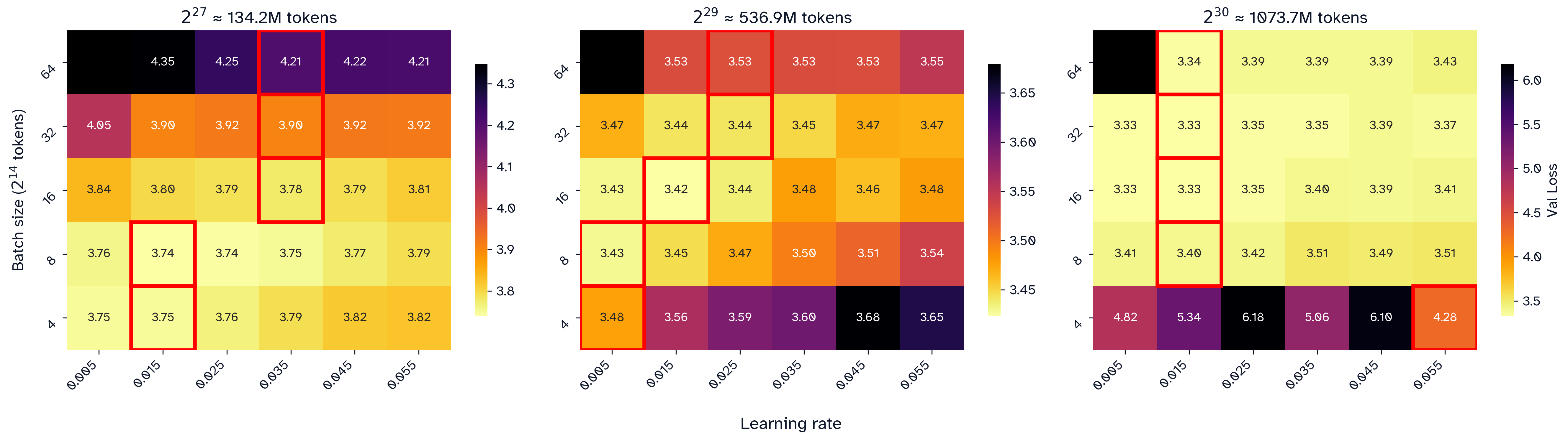
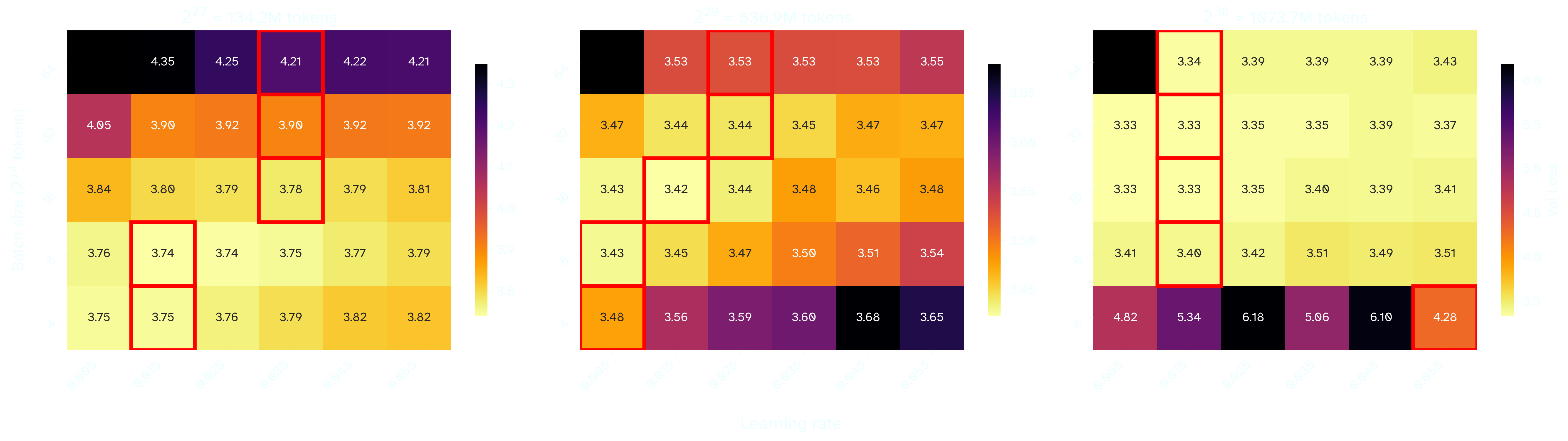
Figure 2: Sweeping Modded NanoGPT at a learning rate x log(batch size) grid at three different token budgets. The lowest loss per batch size is selected in red.

At token budgets of $\approx 134M$, $536M$, $1073M$ tokens, the optimal learning rate seems to converge around $\eta \approx 0.035$, $0.025$, and $0.015$, respectively. Note that $B=4\times 2^{14}$ does not appear to converge at the highest token budget for any of the swept learning rates.

The learning rate appears to increase until around $B<32\times 2^{14}$ tokens, though convergence appears to be faster at higher token budgets. In general, higher token budgets are less sensitive to differences in learning rate or batch size:

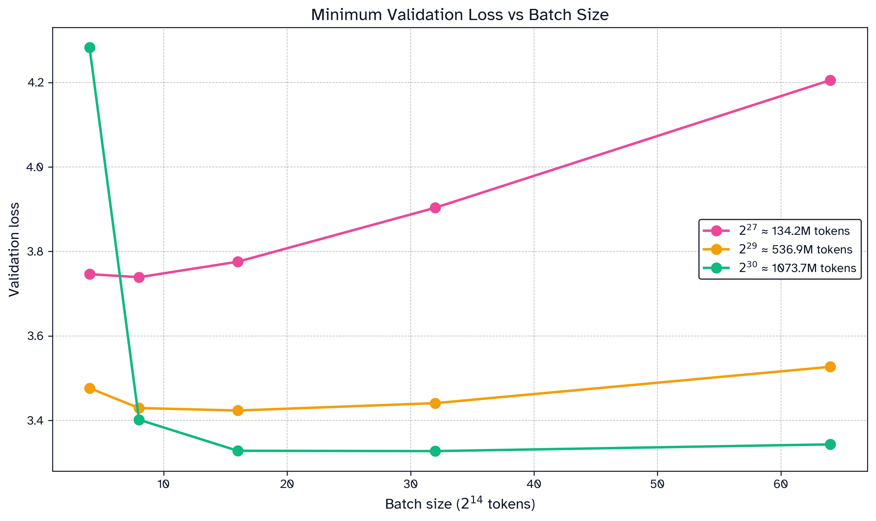
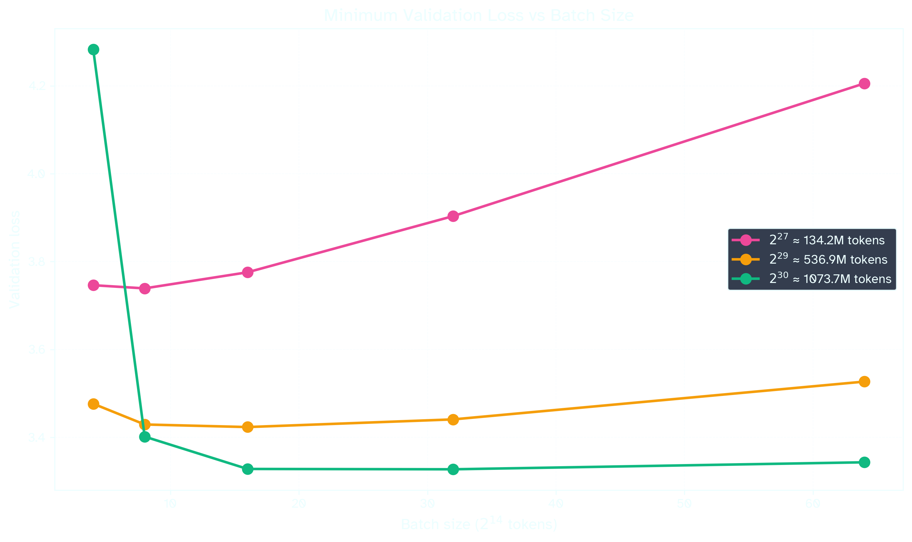
Figure 3: Results from the previous sweep (Fig2) while choosing the optimal learning rate for each batch size. For a fixed token budget, increasing batch size will tend to decrease final validation loss. $B_{\text{critical}}$ is the highest acceptable batch size given some tolerance for loss.

The above graphs demonstrate stability in the critical batch size, especially at higher token budget. Consider the flatness in the curve for the highest token budget ($\approx 1T$ tokens): $1024$ steps at a batch size of $2^{20}$ tokens converges to nearly the same loss at $1024$ steps as a batch size of $2^{18}$ tokens in $4096$ steps. A paper from Essential AI conducts this experiment at larger scales, validating that Muon’s critical batch size is stable and higher than Adam’s. ²⁵

Batch size can often be safely increased over the course of training ¹⁸. Conceptually, this may be because early training focuses on common patterns, so even small batches provide strong gradient signals. Later training involves learning rarer patterns. These sparse signals remain noisy even at high batch sizes, so the batch size can be increased without saturating the gradient. Notably, two strong models trained with Muon, Kimi K2 and GLM 4.5, both increase batch size mid-training ^{26 27}.

Modded NanoGPT’s recent record uses batch size scheduling in order to maximize token efficiency throughout training, decreasing train time by $\approx 1.7\%$ ²⁸.

(3) Faster orthogonalization: Polar Express and beyond

The Newton-Schulz iterative algorithm approximates orthogonalization via a quintic polynomial iteration. This iterative approach is agnostic to the conditioning of the underlying matrix. However, since the matrix becomes better-conditioned over iterations, you can find an optimal polynomial per-iteration, which results in faster convergence. Ansel et al provide optimal coefficients at each iteration step via their algorithm Polar Express ²⁹.

Last month, a paper from Shulgin et al demonstrated that a more precise orthogonalization improves Muon convergence, especially when accompanied with appropriate learning rate tuning ³⁰:

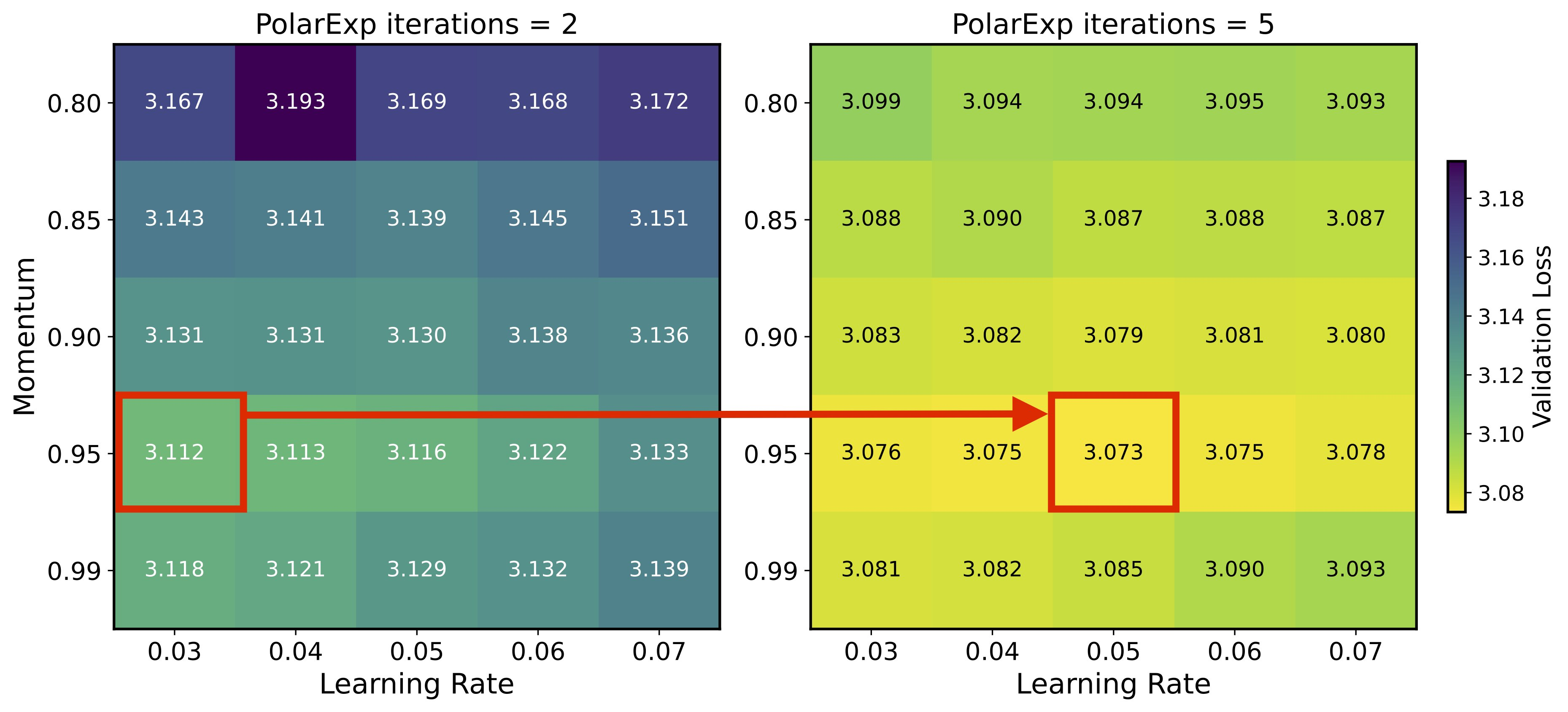
Figure 4: Validation Loss at two levels of convergence for orthogonalization. Shulgin writes “the optimal learning rate couples with approximation quality”, so “higher precision → higher optimal LR + wider stability”

It follows that using Polar Express over Newton Schulz represents an improvement in convergence, and using it led to a new record in Modded NanoGPT.³¹

On ongoing effort in the Modded NanoGPT speedrun is being made for even faster orthogonalization via Almost-Orthogonal Layers, though this has not been incorporated yet.³²

(4) Cautious weight decay

Weight decay is important for large-scale training with Muon. The Kimi team writes: “While vanilla Muon initially converges faster, we observed that some model weights grew too large over time, potentially limiting the model’s long-term performances. Adding weight decay addressed this issue - the results demonstrate that Muon with weight decay outperforms both vanilla Muon and AdamW” ²⁶.

At the relatively small scale of Modded NanoGPT, however, weight decay was doing more harm than good. Weight decay typically involves a tradeoff between immediate convergence and long term stability. In October, a variant of weight decay known as cautious weight decay was proposed ³³, which only decays parameters that will increase in magnitude in the update step:

def apply_update(param, update, learning_rate, weight_decay):
	mask = (update * param) >= 0
	update += weight_decay * param * mask
	return param - learning_rate * update

Algorithm 2: Cautious weight decay (difference from decoupled weight decay highlighted).

Cautious weight decay avoids shrinking weights that are already being moved toward zero by the gradient, so you avoid over-regularizing parameters that are actively decaying. This technique proved effective in Modded NanoGPT. Using cautious weight decay with a decaying schedule improved the record by $\approx 1.3\%$, with final weights $\approx 15\%$ smaller in magnitude than in the unregularized case. ³⁴

(5) Distributed and efficient computation

The implementation of Muon has been optimized in order to distribute the implementation over 8 devices. First, there are several tricks used to speed up orthogonalization over the basic Newton-Schulz algorithm:

• Parameters of the same shape are stacked together so that orthogonalization is vectorized.³⁵
• Additionally, the attention weights qkvo are concatenated so that they are the same shape as the MLPs.³⁶ One MLP is transposed so the input and output MLPs have the same shape.³⁷ This allows attention and MLP weights to be stacked.
• The Newton-Schulz iteration involves the manipulation of symmetric matrices. Using this fact can cut down the number of computations in half for parts of the iteration. Custom triton kernels have been written for these steps. ³⁷

Second, there are a few tricks to distribute the Muon step over all the GPUs:

• Each GPU receives an equal subset of the parameter gradients (via a reduce-scatter).³⁸
• Each GPU processes gradients in groups. Each group is padded to have a “nice” number of parameters, i.e. a multiple of $8$, which is important for underlying kernels.³⁶³⁹ The processing of each group is highly vectorized.⁴⁰¹⁷
• The groups are handled asynchronously so that gradients are being communicated across GPUs while other gradients are being processed inside the GPUs.⁴¹⁴²

For additional information I direct you to Larry Dial’s blog post ⁴³ and the Modded NanoGPT repo.

(6) Conclusion

I hope this post is broadly useful for pretraining with Muon. I want to highlight some important considerations for the Modded NanoGPT recipe:

• The model is small (<124M active params) and has a unique architecture.
• Adam is used instead of Muon on a few parameters: the linear output head, the embedding layer, and a few scalar constants, though this is “standard” for Muon.
• Adam is stepped with twice the number of gradient accumulation steps as Muon. Effectively, it has a 2x batch size than Muon. In the experiment in Section 2, I’ve scaled the Adam learning rate according to the square-root law.

If you are considering using Muon for pretraining, I recommend trying the methods in this post. In summary,

1. You may find an adaptive variant of Muon to be highly effective.
2. You should consider generously increasing the batch size throughout training.
3. Adopt Polar Express instead of Newton-Schulz as your matrix-sign function.
4. When using weight decay, test a simple variation (cautious weight decay) for improved convergence.
5. Significant time can be saved by overlapping computation between gradient computation and computation. If your device can fit them, batch parameters together in the matrix-sign iteration.

I hope in the near future some of these changes will appear in the model training recipes of frontier models, or will be integrated in widely-used libraries containing Muon, such as PyTorch or Dion. Simultaneously, I expect that the Muon optimizer will continue to mature rapidly, with the most effective tricks finding their way into the Modded NanoGPT speedrun.

This post summarizes the work of many records by many people on the Modded NanoGPT speedrun. Section 1 primarily corresponds to a record added by an author of NorMuon, Zichong Li. Sections 2, 3, and 4 correspond to records added by myself, mostly through trying the work detailed in the referenced papers. Section 5 is the result of many people over many iterations, though especially from Larry Dial in the last few months.

---

Thank you to Prime Intellect, who sponsors my research with GPU credits. If this blog post was useful for you, you may cite:

@misc{
	srivastava2025,
	author = {Varun Srivastava},
	title = {Muon in Modded NanoGPT},
	year = {2025},
	url = {https://varunneal.github.io/essays/muon}
}

Footnotes

1. Keller Jordan et al 2024 Modded NanoGPT. The competition is for “the fastest algorithm to use 8 NVIDIA H100 GPUs to train a language model that attains 3.28 cross-entropy loss on the FineWeb validation set.” ^

2. Keller Jordan 2025 The reason I didn’t write a proper arxiv paper for Muon is because I simply don’t think there’s any relationship between the ability to publish a paper with lots of good-looking results about a new optimizer, and whether that optimizer actually works. I only trust speedruns. ^

3. Li et al 2025 NorMuon ^

4. Si et al 2025 AdaMuon ^

5. Zhang et al 2025 AdaGrad Meets Muon ^

6. Frans et al 2025 What Really Matters in Matrix-Whitening Optimizers? ^

7. An et al 2025 ASGO ^

8. Every matrix corresponds to an ellipsoid-like transformation. Orthogonalization makes the underlying ellipsoid into perfect sphere. More formally, the spectral theorem tells us that any matrix transformation can be decomposed into a rotation/reflection + an ellipsoid transformation + a rotation/reflection. This is exactly what the singular value decomposition $A=U\Sigma V^{⊺}$ is describing ($\Sigma$ is the ellipsoid transformation, $U$ and $V$ are unitary matrices). $\Sigma$ is a diagonal matrix, and its entries are called the singular values. A spherical transformation will have singular values all equal to $1$, and the its matrix will be orthogonal/semi-orthogonal (if it’s rectangular). ^

9. Cohen et al 2024 Understanding Optimization in Deep Learning with Central Flows, with a shorter accompanying blogpost here. ^

10. Kustner et al 2024 Heavy-Tailed Class Imbalance and Why Adam Outperforms Gradient Descent on Language Models ^

11. Kovalev 2025 Understanding Gradient Orthogonalization for Deep Learning via Non-Euclidean Trust-Region Optimization ^

12. Anonymous ICLR Conference Submission 2025 Long-tailed Learning with Muon Optimizer ^

13. Weijie Su 2025 Isotropic Curvature Model for Understanding Deep Learning Optimization ^

14. An earlier footnote explains why orthogonalization makes the update “well-rounded”. This prevents steps that are too steep in any direction, which may help to avoid “sharp minima”. Another geometric intuition for orthogonalization is conveyed in Bernstein and Newhouse 2024. To summarize, SGD will update the weights away from the gradient with magnitude corresponding to the distance in the Euclidean metric. It turns out that the correct metric for the gradient is actually the spectral metric, e.g. with respect to the transformation. Orthogonalization acts as a map (“dual map”) from transformation space to weight space. This aligns the geometry of the update with the geometry of the weight space. Another geometric intuition I have is by instead considering the effect of orthogonalization on the weights: if each update is orthogonal (all singular values are $1$), the weights themselves will be well-conditioned (singular values will be somewhat near $1$). This is demonstrated in practice (see Damek and Deusvyatskiy 2025 and Boreiko et al 2025), even though orthogonalization is of course approximate. We can therefore view Muon as effectively performing gradient descent down a constrained submanifold of the full parameter space. Understanding Muon as descending down this manifold, where all its points are well-conditioned matrices, helps me visualize why Muon can avoid ill-conditioned minima. Along these lines, Jeremy Bernstein has proposed Manifold Muon, which tweaks Muon such that the weights remain orthogonal throughout training. ^

15. In fact, the columns are the output singular vectors weighed by the input singular vectors. The orthogonalized update is just a rotation matrix that aligns the input space with the output space. The column-wise RMS therefore tells us how much how much the input neuron contributes to the output spectral direction. ^

16. Li 2025 Modded NanoGPT Record 41 ^

17. Srivastava 2025 Modded NanoGPT Record 42 ^ ^

18. Ai2, Merrill et al 2025 Critical Batch Size Revisited ^ ^

19. McCandlish et al 2018 An Empirical Model of Large-Batch Training ^

20. I’m being somewhat imprecise with how we define the signal to noise ratio. McCandlish et al ¹⁹ defines a critical batch size $B_{\text{noise}}=\text{Cov}(G)/\mathbb{E}(G{)}^2$ for their analysis of SGD. I’m using its inverse as the SNR. ^

21. Granziol et al 2020 Learning Rates as a Function of Batch Size contains a proof. ^

22. Li et al 2024 Surge Phenomenon in Optimal Learning Rate and Batch Size Scaling ^

23. Jianlin Su 2025 Rethinking Learning Rate and Batch Size (Part 3): Muon ^

24. Simo Ryu 2025 Adam vs Shampoo vs Muon on MNIST. all follow the lr ~ sqrt(BS) law. ^

25. Essential AI, Shah 2025 Practical Efficiency of Muon for Pretraining. ^

26. Moonshot AI, Liu et al 2025 Muon is Scalable for LLM Training ^ ^

27. Zeng et al GLM-4.5 ^

28. Srivastava 2025 Modded NanoGPT PR#163/Record 46 ^

29. Ansel et al 2025 The Polar Express ^

30. Shulgin et al 2025 Beyond the Ideal: Analyzing the Inexact Muon Update. Corresponding tweet thread here. ^

31. Srivastava 2025 Modded NanoGPT Record 38 ^

32. Thibaut Boissin 2025 Modded NanoGPT PR#155 ^

33. Chen et al 2025 Cautious Weight Decay ^

34. Srivastava 2025 Modded NanoGPT Record 43 ^

35. Cesista, Maddox et al 2025 Modded NanoGPT Record 20 ^

36. Dial 2025 Modded NanoGPT Record 36 ^ ^

37. Xu 2025 Modded NanoGPT Record 27. The symmetric kernels are also part of the Dion repository. Note that a similar technique was earlier proposed and implemented in CUDA (Flash-Muon). ^ ^

38. Jordan 2024 Modded NanoGPT Record 6 ^

39. Dial 2025 Modded NanoGPT Record 40 ^

40. Romera-Paredes, Hive AI 2025 Modded NanoGPT Record 32 ^

41. Willeke et al 2025 Modded NanoGPT Record 22 ^

42. Yang 2025 Modded NanoGPT Record 23 ^

43. Larry Dial 2025 How the NanoGPT Speedrun WR dropped by 20% in 3 months ^